
Time Series Forecasting for Arrival Temperatures
Sometimes physics-based approaches are not possible


Background
Time series modeling is widely used for a vast array of applications, ranging from predicting consumer market trends to forecasting field behavior. Following up on our previous article about time series forecasting, this piece aims to explore the complexities inherent in this domain and then present a real world example of applying time series forecasting to help predictions in a gas field.


Complexities with Time Series Modeling
Unlike classical regression or classification tasks, time series modeling involves temporal dependence among observations, meaning each observation is influenced by preceding time intervals. This requires a different approach to data engineering, training, and deployment. This article lists some of the main issues with time-series modeling when starting with a machine learning approach. These can be summarized as follows:
Time series models require constant re-training before predictions because under-lying data distributions are expected to change during forecasting
Conventional train/test splits are not suitable in most cases, especially when you don’t have a lot of data points (as we will see further below, consider 2 years of monthly data - you could only have 24 data points to work with!)
Forecast uncertainty should be quantified as much as possible (since all forecasts will be wrong to some extent)
Keeping these in mind, it is useful to understand one of the most proven modeling techniques in the domain of time series, SARIMA, which stands for Seasonal Autoregressive Integrated Moving Average. It is an adaptation of the original ARIMA model to account for seasonality. Breaking these terms down:
Autoregression (AR): An observation at a particular time is dependent on observations from previous time steps
Integrated (I): Time series is made stationary by subtracting an observation from a previous observation
Moving Average (MA): An observation depends on the moving average applied to previous observations
The ARIMA model components are specified as 3 integer parameters. The SARIMA version adds another 4 integer parameters to then account for autoregression, differencing and moving average of the seasonal components and the number of time steps for a single seasonal period.
Case Study for a Gas Network
Recently, we worked on forecasting temperatures at a node in a complex gas condensate network with 100’s of miles of pipelines. These temperature predictions are crucial for understanding the potential liquid drop out, which in turn affect sales and revenue forecasts.
Typically, in a problem such as this we would use a physics-based simulation model like OLGA because understanding the underlying physics can help overcome uncertainties on how system changes will affect key results. However, in this case, OLGA is prohibitive because of the following reasons:
100’s of pipelines spanning 100’s of miles leads to large run times. This is further exacerbated by needing to run the simulation sufficiently long to capture significant transients that occur in the system and return a true representative average temperature. The end result is a simulation that takes days to run for just one data point.
Certain pipelines are buried, while others are not. This leads to uncertainty in the true heat transfer throughout the system. Tuning is possible, but to the point above, since each run takes excessively long, this would also be time prohibitive.
All the sources contributing gas to the network have varying compositions, resulting in more or less liquid dropout, which further complicate the thermal behavior.
The issues above led us to take a data-driven approach instead. However, we aren’t in the clear yet…
From an initial data analytics exercise, we know that the two most important variables impacting the system temperatures are the overall gas rate and the ambient temperature. But, each of these features has a unique problem associated with them:
Gas rates - the system is expected to see year-over-year increases in the gas that it transports. This means any data-driven model will by default be extrapolating in its predictions if gas rate is a feature.
Ambient temperature - we don’t actually know what the ambient temperature will be in any given future month or year, which means we must first forecast this variable before being able to use it in our final model. Generally, forecasting one of your features can lead to error propagation. In this case, because average monthly ambient temperature is relatively easily predicted, this risk was deemed to be OK.

The Results
Based on the theory discussed above, our default approach to this request was to utilize a SARIMA model because we are dealing with time series forecasting. However, we have also included a seasonal model without an integration term (SARMA) as well as a simple linear regression model.
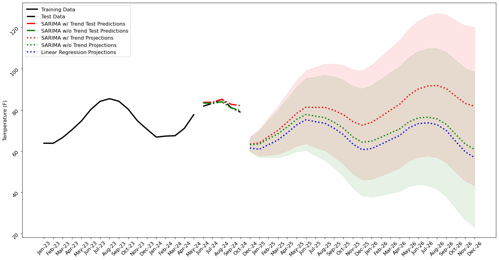
In the plot below, you can see the forecasts predicted by:
SARIMA while accounting for trend in the data (red)
SARIMA without accounting for any trend or SARMA (green)
Linear regression (blue)
Additionally, the uncertainty bands predicted by both SARIMA models are also plotted. These naturally expand as you forecast farther into the future.
Which model is the best?
As we can see in the trends, all models do a decent job at capturing the seasonality associated with varying ambient temperature. However, the SARIMA without trend and the linear model show very little effect from the increased gas rates in the system, which are not shown but do increase by close to 100% in later years. In contrast, the SARIMA model with trend, shows more of an effect of increasing gas rate through the system. The question is which of the forecasts are “correct” (or more appropriately, “less wrong”)?
All 3 models performed acceptably with the test data (RMSE of ~ 3°F). The linear regression predictions, while close to one of the SARIMA models, cannot be blindly trusted as it is predicting on forecasted rates that are outside its training bounds. The time series models also suffer from this same issue in many ways, however, by using a time series model such as SARIMA, we as the engineer can insert our bias into the model and that bias can be derived from our domain knowledge on the topic.
For example, we know that higher rates entering the system are likely to lead to a net increase in the thermal mass of everything in the system. While some lines are unburied, most are buried, which will help preserve that thermal mass. Additionally, we are dealing with a relatively low pressure drop system, where Joule Thomson cooling effects are not drastic. Taking all of the above into account, our intuition is that holding everything else constant, we would expect a net increase in outlet temperatures as total gas rates increase.
From a model perspective, this means that we can justify the “I” (integrated) term in the SARIMA model as we think there is a net increase occurring as time moves forward due to the higher rates.
Which model should we use?
Now, before we pat ourselves on the back too much for picking what we think is the best model, we should remember the quote from the famous statistician, George Box:
“All models are wrong, but some are useful”
While we believe that the SARIMA model is the single “best” model we have, it’s important to revisit the issues with the data mentioned further above. Each of these models are extrapolating on total gas rates the field has never seen before, they are using forecasted ambient temperatures as inputs, and by today’s standards they have a very small training set with just monthly average values for the last year.
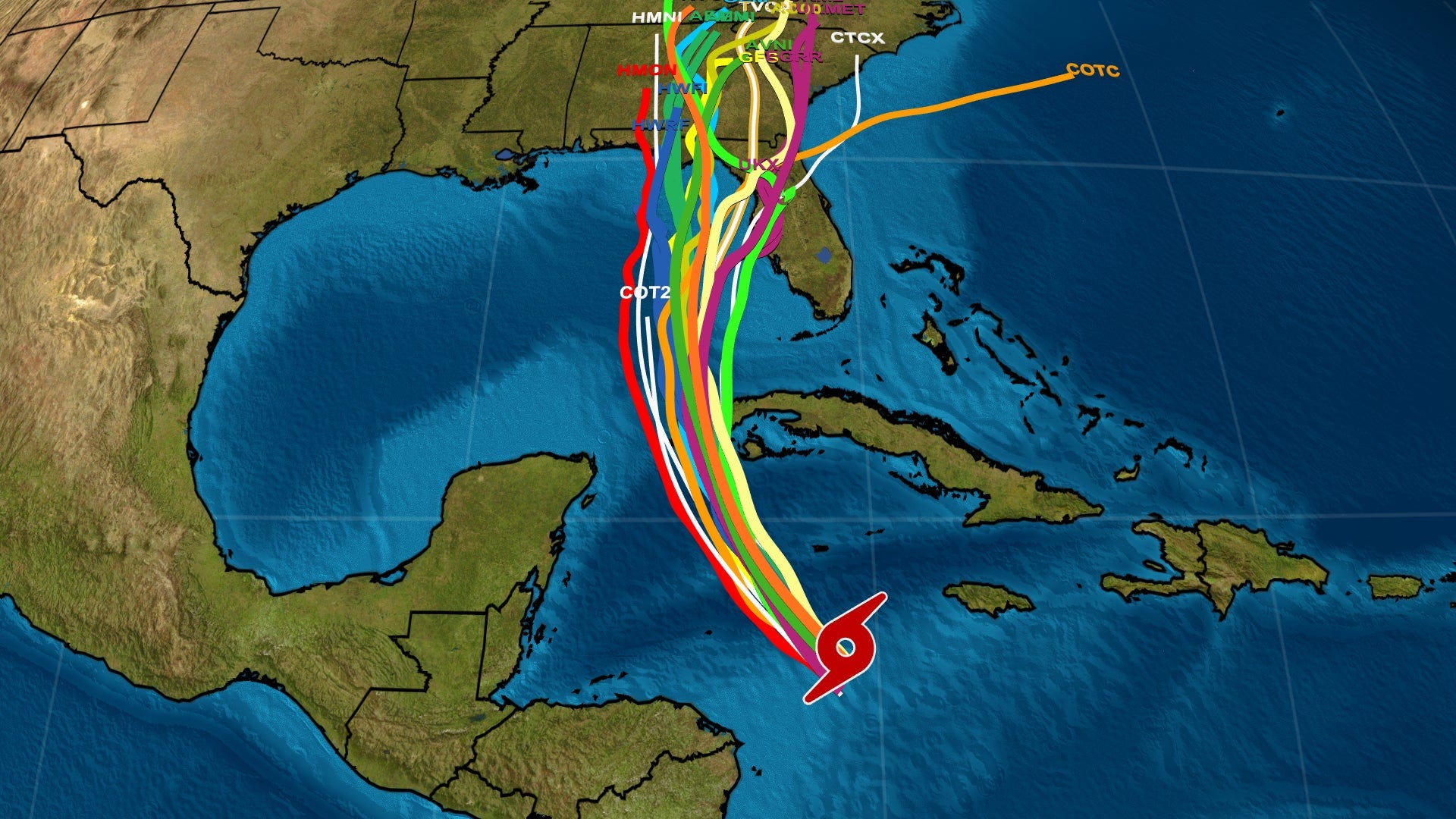
Folks in Houston are no strangers to the hurricane prediction models and spaghetti charts. In this particular use-case, the model we should actually use is likely to be an ensemble of several techniques including SARIMA, linear regression, and even deep learning based methods once more data is available. The “average” prediction from several trained models can often be the best choice, and for that reason we will keep all these models available in our forecasts.
As new data comes in each month, our various models will be automatically re-trained to provide the latest forecasts on temperatures for the client. Each time this occurs, we expect to be producing more accurate forecasts than the previous month.
Conclusions
Time series modeling needs to be handled with care. There are complexities involved which require tailoring your data cleaning, training and deployment pipelines. A simple baseline to start with is the SARIMA (or ARIMA if your use case does not have seasonality) model. Always set these models up for re-training because you have to expect underlying data distributions to change in deployment.
And finally, in a world with so many tools at your disposal, it’s important to understand the strengths and weaknesses of various approaches, whether that be physics-based vs. data-based models, or sub models within each of those areas.
When you are a hammer, everything looks like a nail. But if you are an entire workshop, then everything looks like a problem you can solve.
This is our philosophy at Pontem - ensure you have numerous tools in your tool belt and know when it is best to use each one.