
The Physics Behind Hydrate Dissociation
A Picture Is Worth 10 Million Equations

Our recent post examined some practical examples for hydrate remediation in oil and gas production systems. We continue our discussion with hydrate dissociation and the science behind melting hydrates. Whether you’re a geeked out nerd like me, or you are just mildly curious about how things work you probably instinctively know some of the concepts. It’s why you prefer big ice in your whiskey but not in your flow line.

Fundamentally, nothing changes in the thermodynamics when dealing with hydrate formation or dissociation, and models are quite clear in determining stable or unstable hydrates for a given system. There are several models to evaluate the thermodynamics of a system that are accepted as standards in the oil and gas industry, such as Multiflash, PVTSim, and CSMGem.
Chemicals will shift the equilibrium curve. Depressurizing the system or providing latent heat will move the system’s thermodynamics relative to the hydrate equilibrium curve. One must, obviously, consider kinetics when asking how quickly a hydrate plug will form or melt. Colorado School of Mines Hydrate Plug Dissociation Tool (CSMPlug) predicts how quickly a hydrate plug will dissociate by solving transient heat-transfer and moving boundary (Stefan-type) problems with hydrate thermodynamic equilibrium constraints.
This post will provide an overview on the principle mathematic equations to solve the “how long” question and we’ll look at some examples to highlight how this may apply in the field.
Math Is Everywhere
As one may imagine, hydrate dissociation kinetics is quite dynamic and there is not a single equation to describe this process. Within CSMPlug, for example, there are multiple equations coupled together: transient cylindrical heat conduction, hydrate equilibrium thermodynamics, moving boundary, latent heat balance, and prescribed pressure history.
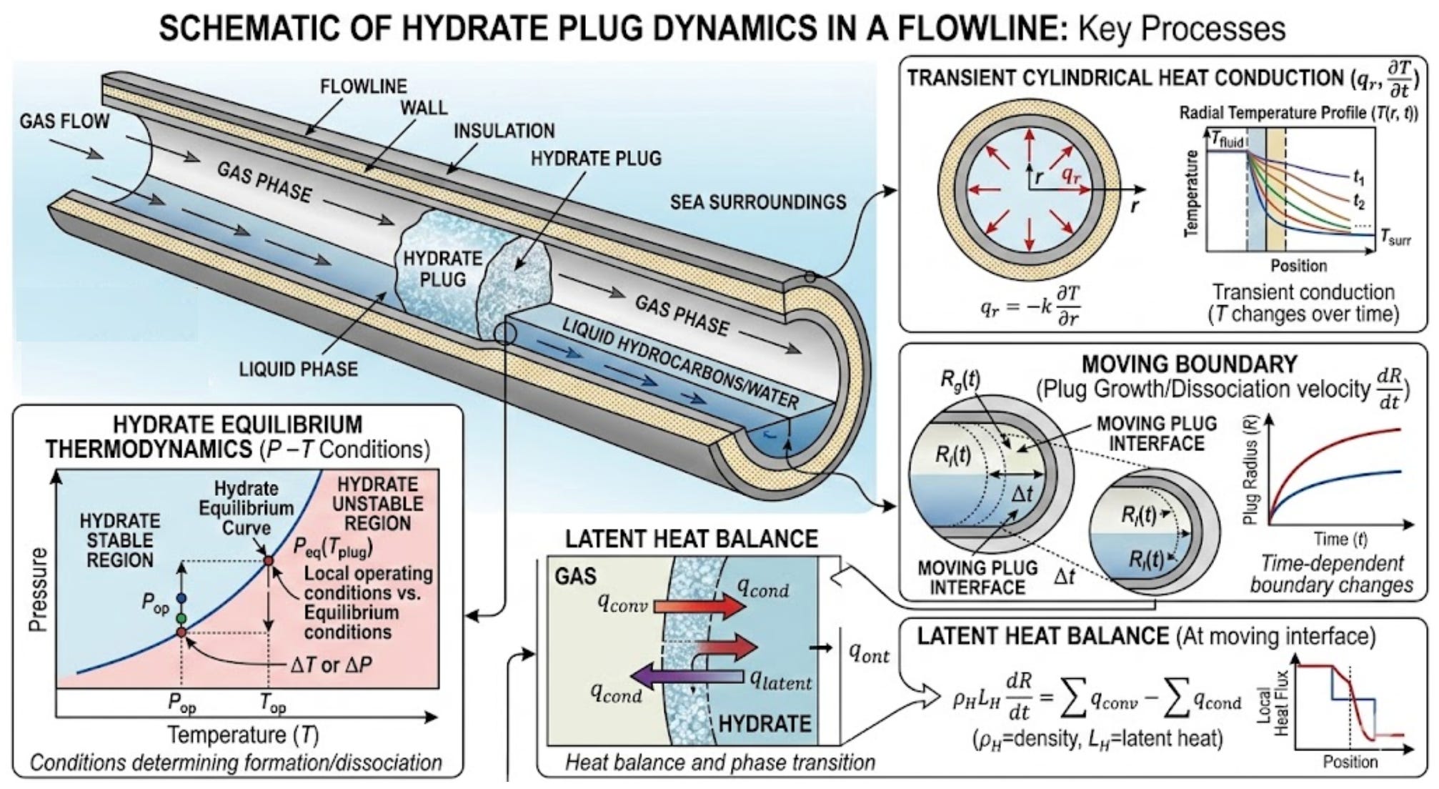
The model works by solving heat conduction at the surface of a hydrate cylinder while estimating dissociation due to temperature changes and pressure drops. Then it predicts how long these changes will take to fully dissociate the solid hydrate plug at the boundary. Once enough heat has been put into the system to fully dissociate hydrates at the surface, a new boundary is set with a smaller radius. This process continuously repeats until the plug is fully dissociated. Two limitations within the model are it does not simulate axial convection nor consider fluid flow dynamics (which makes sense to put this limitation in place as the hydrate plug is typically immobile!). In other words, the dissociation front moves radially inward as conditions change.
Math Fun (don’t worry, it’s Type 2 fun)
For a given hydrate plug, the series of continuously solved equations include:
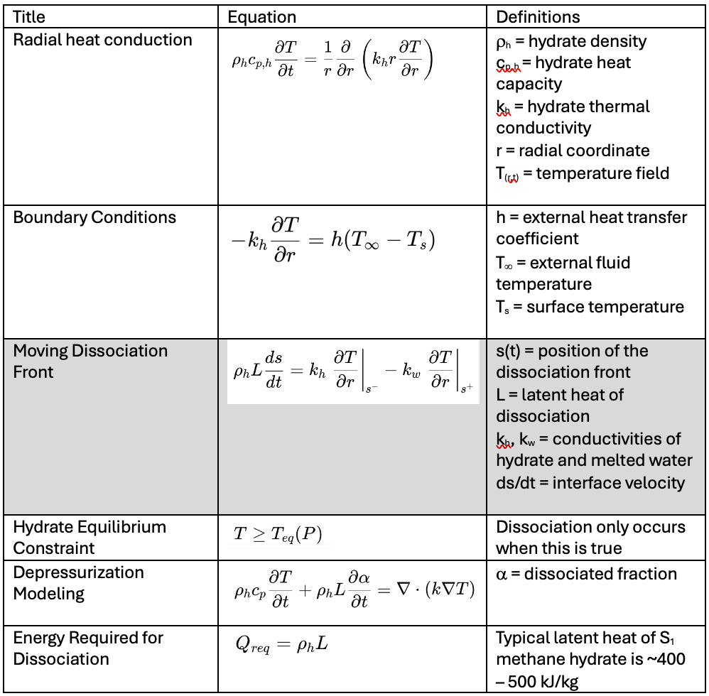
A critical component for this model (and really the equation that determines how fast the hydrate dissociates) is at the phase boundary (shaded equation in the table), which is moving. The final solution is presented (hydrate is fully dissociated) when
s(t) = 0
What does this mean?!
For a hydrate plug, dissociation rate is controlled by Heat flux vs Latent heat requirement.
If the heat supply is small then dissociation is slow, which is the case if the flow line is insulated. A primary example of this that many will be (unfortunately) familiar with is melting a hydrate via depressurization alone. A flow line with a hydrate plug may begin with a dual-side depressurization, which initially takes the surface of the plug outside the hydrate equilibrium curve. There is an initial rapid dissociation (at the hydrate surface). However, this is an endothermic reaction and temperatures decrease locally (at the new surface) because heat is absorbed. This forces the conditions back across the equilibrium curve and hydrates are once again stable. The temperature can only warm up from heat provided from outside the flowline. If this is subsea, it will not warm up very much and will do so slowly. If the line is insulated, then that process is even slower.
This is why depressurization-only remediation can take several weeks in a subsea system with an insulated flow line. The seabed temperature is cold and does not provide much heat to the system and the U-value of the insulation severely limits the transfer of thermal energy.
Do I Really Need A Fancy Model For This?
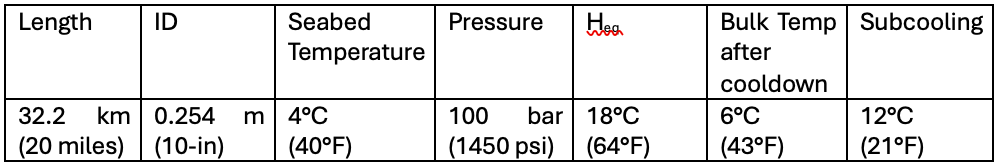
There are sound engineering first-principle calculations out there, so won’t those work? That’s a great question. Let’s go through some examples and compare. Let’s look at a hydrate plug that has formed in a 20-mile subsea tieback. Here’s the system:
Let’s assume a 50 m full-bore plug forms in the line. The volume of this plug can be calculated as
V = (pi)r2L = p(0.127)2(50) = 2.54 m3
We’ll also assume hydrate density to be ~900 kg/m3, so the mass of the hydrate is 2,286 kg. This is a very conservative estimate, as it assumes 0% porosity and full conversion of hydrates (no free water/gas within this volume).
First Principle Calculations for Depressurization
As mentioned previously, depressurization is a viable method to dissociate hydrates because depressurization makes hydrates thermodynamically unstable. However, dissociation absorbs latent heat (it is an endothermic process and is self-cooling). After the initial flash dissociation, the plug temperature drops toward equilibrium. The heat to warm the system back above equilibrium temperature must then come from the surrounding seawater through a layer of insulation.
The heat flux from seawater is estimated by considering the surface area around the plug:
A = 2(pi)rL = 2pi(0.127)(50) = 39.9 m2
If we assume an insulted pipeline, h = 8 W/m2K (1.4 BTU/hr.ft2.°F), and a small driving force after depressurization (DT = 5°C) then,
Q = hADT = 8 x 39.9 x 5 = 1,596 W
Assuming the latent heat of a methane hydrate is 450 kJ/kg then the energy required to melt the hydrate is
Qtotal = 2,286 x 450,000 = 1.03 x 10⁹ J
The dissociation time calculation becomes
t = (1.03 x 10⁹) / 1,596 = 645,000 sec = 179 hours = 7.5 days
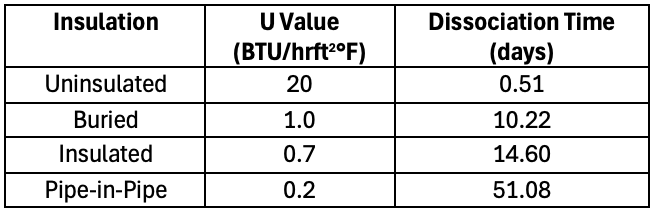
If there is a more effective insulation and the heat transfer value is only 3 W/m2K (0.52 BTU/hr.ft2.°F), the dissociation time increases to 20 days. Technology giveth and technology taketh away! What was preserving thermal energy from the reservoir to carry along the flow line is now severely limiting thermal transfer from the seabed temperature into the system. This obviously helps to reduce the risk of hydrate formation, however once hydrates are present the remediation becomes more challenging. The chart showing various flow line insulations below highlights the differences and drives the point home.
Another important factor to consider is when pressures become very low (for a subsea tieback). Let’s consider a system that has managed to be blown down to 150 psi. The hydrate equilibrium temperature for Green Canyon Gas (a representative Gulf of America gas composition) is shown below. At equilibrium the system will slowly warm to 40°F by the surrounding ambient temperature, which will melt the hydrates. This will, in turn, cool the system down below freezing temperatures. The operation then risks ice formation!
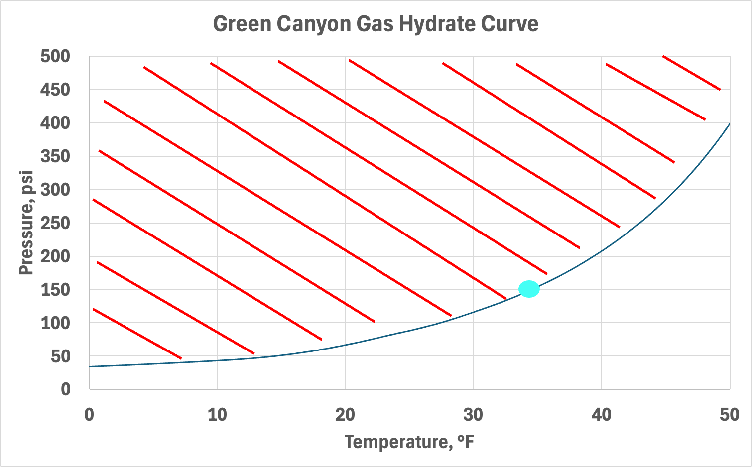
This Catch-22 practical example is one reason why there are usually additional methods that are used in parallel for hydrate dissociation when depressurization is employed, which we’ll discuss below.
First Principle Calculations for Direct Electrical Heating
If we consider DEH for our dissociation example and assume 150 W/m is applied to the flowline, the total heating power applied to the hydrate plug is
P = 150 x 50 = 7,500 W
Let’s also assume there is only 85% effective heat applied, so P = 6,375 W. The same energy is required to dissociate the hydrate, which makes the time requirement
t = (1.03 x 10⁹) J / 6,375 W = 161,568 sec = 1.9 days
Obviously, reducing deferred production from 3 weeks to 2 days is a huge advantage. Unfortunately, installation CAPEX and OPEX costs to provide power in order to maintain the system for a 20-mile tieback must be considered against the risk of a hydrate plug occurring (once or multiple times).
How is a model like CSMPlug different from what we just did with first principle calculations?
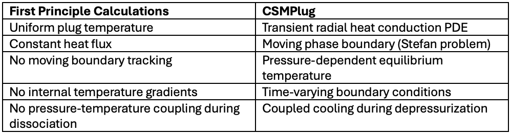
The impact of these differences can be significant. CSMPlug will produce:
· Slower early-stage dissociation (based on internal gradients)
· Nonlinear time evolution
· Self-cooling effects
· Interface motion
The main deviations come down to three main sources:
Internal thermal gradient – In reality a hydrate plug, much like an ice cube in your Manhatten, will melt from the outside inward. While the surface warms relatively quickly, the core remains cold. In our simplified example, the equations assume a uniform plug temperature, constant heat flux, and no moving boundary resistance. There really is an internal thermal gradient where in the early stages the surface warms quickly while the core remains cold. This assumption produces an error ranging + 10 – 25% for the dissociation time.
Self-cooling during depressurization – During a pressure drop, the surface temperature drops, therefore DT shrinks and heat flux decreases. A lumped model assumes a constant DT. This produces a larger error – typically ranging + 20 – 50%.
Variable heat transfer coefficient – As the plug shrinks, the surface area decreases and the contact resistance changes. Our simplified calculations assumed a constant area. This difference accounts for +/- 10 – 20% error.
Long plug lengths – For very long plugs, pressure gradients matter more and dissociation may start at the ends. Lastly, melt rates are not uniform. A simplified model will under or over predict the dissociation time by up to 2x in some cases.
The first principle calculations tend to break down when considering hydrate plugs that form in subsea tiebacks because:
· Strong depressurization (large subcooling)
· Thick insulation
· Very low external DT
· Thick plugs (> 0.2 m radius with low conductivity)
· Partial dissociation with trapped gas pockets
In our DEH example, we estimated 45.6 hrs (1.9 days), whereas incorporating a full Stefan solutions (solid melting to a liquid) will give a solution ranging 52 - 62 hrs (+15 - 35%).
Bonus Topic: Chemical Options
Methanol and MEG (mono ethylene glycol) are often used to prevent hydrates from forming as a thermodynamic inhibitor (THI), and they both can be used to dissociate hydrate plugs. Without going into the thermodynamics too much, a safe approximation for the volume of methanol required for hydrate equilibrium temperature suppression is ~ 0.8°C / wt% MeOH and ~0.3°C / wt% MEG. The concentration component is an important factor to consider because free water is released from the hydrate as it dissociates, which dilutes the inhibitor. In practice this means THI must be continually fed into the flow line to fully dissociate the hydrate. This also means there must be communication across the hydrate plug or else the injection side of the line will keep increasing in pressure and the amount of THI will be limited (or the line will burst!).
In 2024, Koh et al. reported a model to describe a two-step mechanism to dissociate a hydrate plug. In the first step, heat is applied to begin the hydrate dissociation process and create annulus spacing between the pipeline wall and the hydrate plug (images 1 - 3 below; this is critical as one needs to establish communication across the plug). In the second step (images 4 - 6), THI is delivered to one side of the hydrate to accelerate the dissociation of the hydrate.
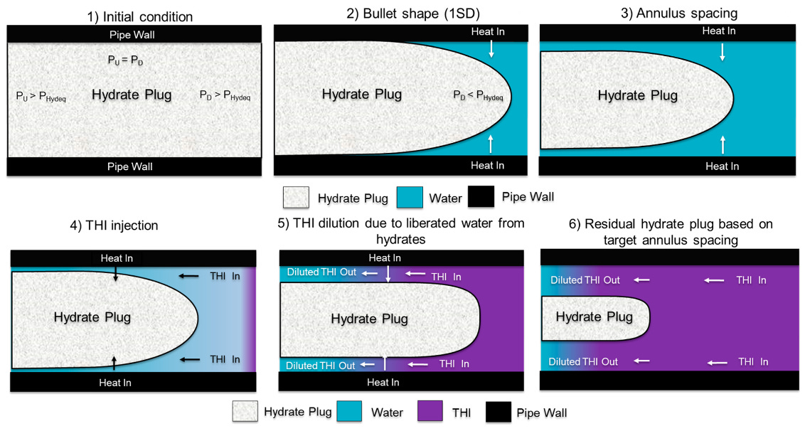
In addition to heat, the annulus spacing can be established through one-sided depressurization. The second step is dependent on the THI concentration gradient. The model calculates the accumulation of water and THI over time based on the dissociation. The model also takes into account the transient axial convection of the THI flow rate and associated thermodynamic changes caused by THI concentration changes. Other considerations include the porosity and permeability of the hydrate plug, heat transfer coefficient, hydrate plug length, and annulus spacing.
When applied to the field, the model predicted a hydrate dissociation time of 1 - 2 days, depending on THI flow rates, hydrate porosity assumptions, and time to create an annulus spacing (shown below).
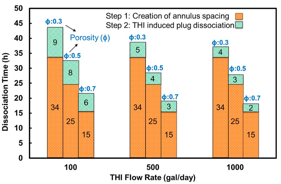
In practice, the field was able to utilize multiple techniques to minimize safety risks and reduce the downtime to a minimum level. The super interesting point of this example is a model was developed to predict what is possible, yet unknown variables still existed: plug length, porosity, and location to name a few. The model validation still worked and by incorporating actual field data the remediation times provide valuable options to get the hydrate safely melted and production up and running.
In other words, the best solutions (in our humble opinions!) come about when combining scientific theory (what’s possible) with actual limitations / real world scenarios (what’s practical).