pypontem : Rolling up your sleeves!

A walkthrough on how to use pypontem

Following up on our post introducing pypontem, here’s a guided walkthrough on key functionality. But before we dive into some serious detail, a word on the design we adopted for pypontem.

As mentioned in our introduction article, currently pypontem is focused on OLGA data processing with more platforms hopefully to come in the future!

Some implementation details

When developing pypontem, we adopted the following structure currently:

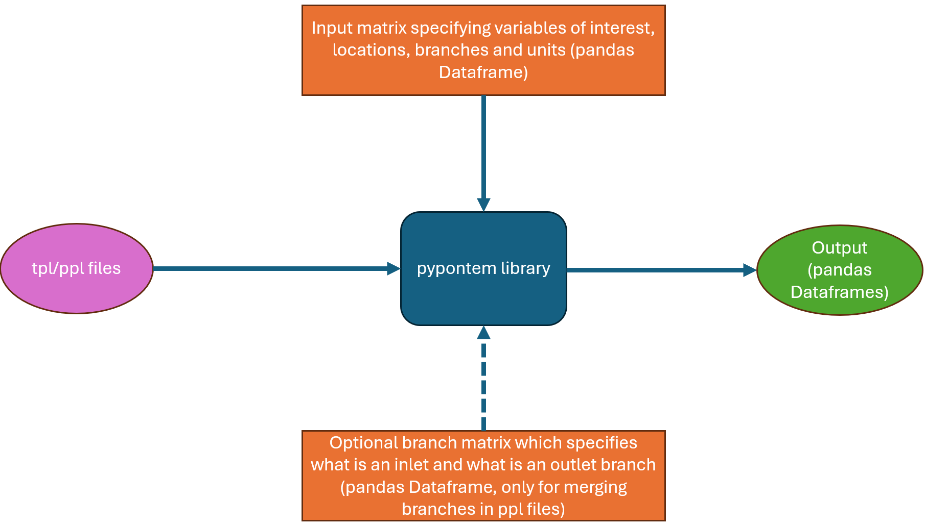
Alongside the tpl/ppl file of interest, we require users to create a pandas dataframe which specifies the variables of interest and information like what units the outputs are desired in. This enables parsing of multiple variables in one go, without having to execute the same function/method repeatedly. Additionally, for ppl files, in order to merge branches, a branch matrix is needed, which specifies what the inlet and outlet is at each node in the model.

Getting started

To recap, to install pypontem, we recommend you create a virtual environment via anaconda/miniconda/virtualenv. In the example below, we are installing a conda environment. NOTE: We recommend you install python 3.12.3 when using pypontem.

# creating the environment 
conda create -n pypontem_env python=3.12.3 jupyter matplotlib 
# activating the environment 
conda activate pypontem_env 
# installing pypontem 
pip install pypontem

Working with single tpl and ppl files

Once you have got pypontem installed, you can open either a Jupyter notebook or write a python script to process your tpl and ppl files. In this section, we will look at single tpl or ppl files.

• Import necessary libraries

  

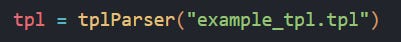
• Specify the location of your file to be processed and initialize the tplParser object

  

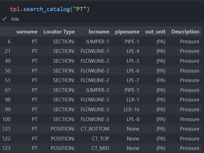
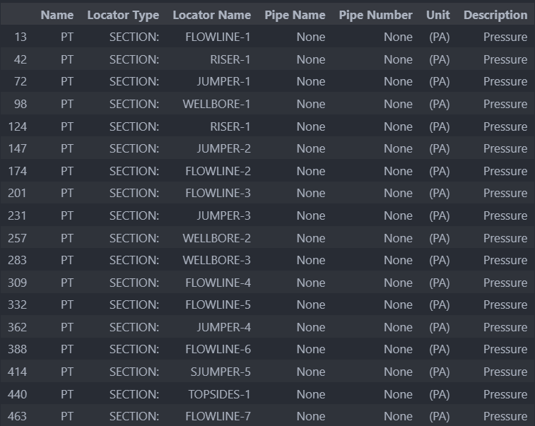
• Search the catalog for the variable of interest. The search_catalog function accepts an OLGA variable name as argument and retrieves all instances of that variable in the provided tpl/ppl file. The result is a pandas dataframe that looks like this.

  

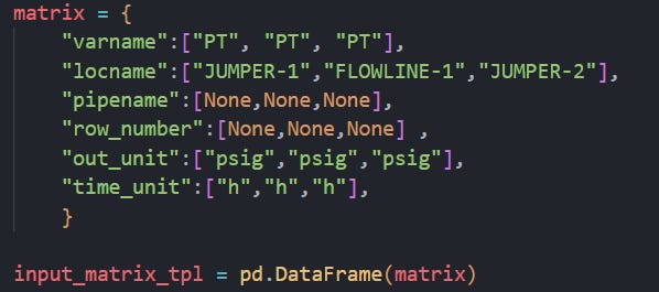
• Then specify an input matrix with the variable name, location name, name of the pipe, number of rows you need out, the unit you want the variable in and the unit you want the simulated time in. This has to be a pandas dataframe. Below is an example of how to do this via a Python dictionary. You can also create a csv file and read it through pandas if that’s your preferred way. NOTE: If you are using a dictionary the keys will have to be named exactly as shown below and if you are using a csv file, the column names should be the same names as these dictionary keys

  

• You can extract the information from the tpl file using the extract_trend method of the tplParser class. This returns a pandas dataframe. In the below example, we are going to use this dataframe directly to create plots using matplotlib

• The calc_average function is a helper method which lets you calculate averages from the trends extracted from a tpl file. It requires the input matrix and the averaging method as arguments. There are a few averaging methods you could use. You could specify the start and end points (say, from the 1st to the 5th point) like so:

  

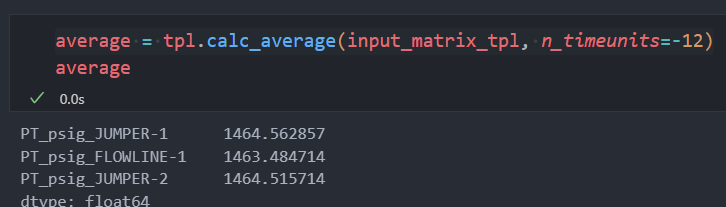
• Or you could specify the number of time periods you need to average over (this will need to match the entry in the time_unit column in the input_matrix). In the example below, we are averaging over the last 12 hours:

  

• Or over the first or last x rows of data as below:

  

Moving onto ppl files,

• You initialize the pplParser with the file path to the ppl file

  

• Look up the details of the variable you are interested in extracting from the catalog

  

• You specify your input matrix. Note, the extra key/column names needed for ppl profiles. branchname to specify the name of the branch, out_unit_profile to specify the length/geometry unit, start_time to specify at what simulation time you want to start extracting from and end_time to specify at what simulation time to stop extracting.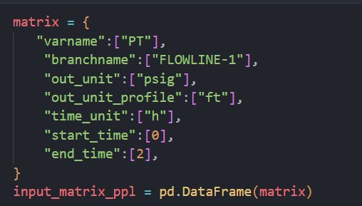

  

• You extract the profile data using the extract_profile method as below:

  

• The returned pandas dataframe will have a structure similar to below. The first column is the geometry/length, the second is the variable at the start time and the third, in this case, is the variable at the end time. If you have more than 1 step between start and end, they will be structured in their own columns in ascending order of time.

  

• And, you can create plots with matplotlib, like below:

  

• A useful functionality we added was the ability to merge branches. You need to specify a branch matrix like below. The below example can be read as Jumper-1 flows into Flowline-1 which flows into Jumper-2. After you define the branch matrix, use the extract_profile_join_nodes method to merge branches. Note, when merging branches, you need to make sure the branches are also listed in the input_matrix.

  

• The returned dataframe would have a similar structure as below:

  

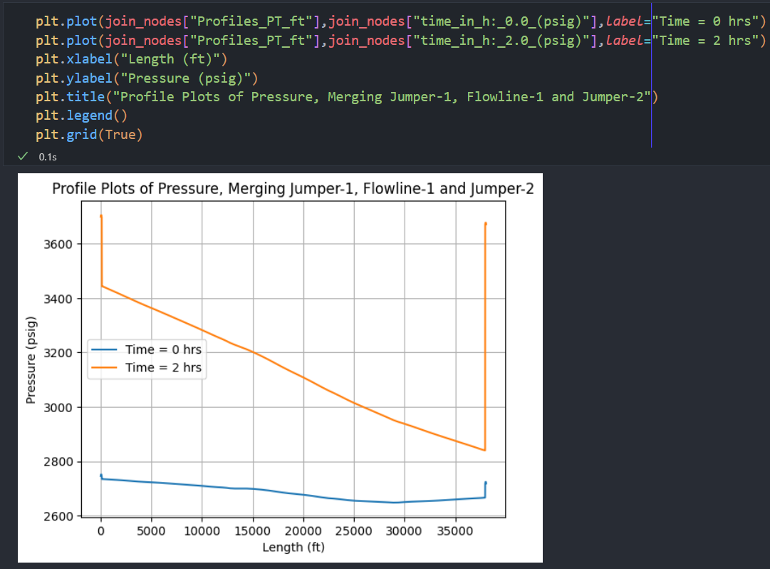
• Which you can plot with matplotlib or any other plotting library you like

  

  Working with batch files

  We have two classes named tplBatchParser and pplBatchParser which can handle batches of files. For illustration purposes we have duplicated our example tpl and ppl files to simulate a batch.

• For tpl batch parsing, import the tplBatchParser class and initialize it with the filepaths of your tpl files.

  

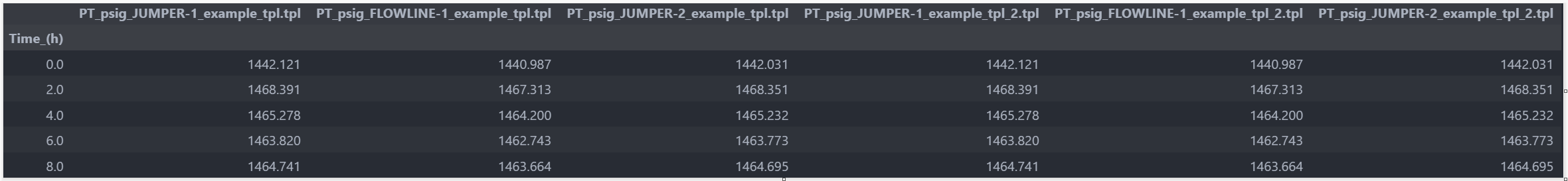
• Once the batch parser has been initialized, you can extract trends and view the returned pandas dataframe like below. Note that the column names have the filenames appended to distinguish which column belongs to which file.

  

  

• You can also calculate averages from a batch with the calc_averages method in the tplBatchParser class

  

• The pplBatchParser class works similarly, as shown below:

  

• Merging branches in a batch of ppl files works similarly to how the pplParser handles merging for a single file. This is shown in the code snippet below (again, the file names are in the column names

  

There’s more!

In addition to the key functionality described here, there are more helpful features in pypontem, alongside Jupyter notebooks you can download in the official docs and the official github repository.