
Into the Matrix
Solving Flow Assurance problems for CCS developments using one of OLGA's newest features, the NEO solver


Here’s a result from one of our recent CCS models that has no business being true:
Make the surroundings colder, and the CO₂ arrives at the bottom of the riser hotter, not colder.
I’ll say that again: cooler outside, warmer inside.
Every instinct you have says that’s backwards.
Is it real? Is it a modeling artifact? Or is it a glitch…in the Matrix?
Is what I’m seeing real, and if so, why? That one question is a recurring theme that runs through everything we’ve been doing on a client’s strategically important CCS project. So, grab a coffee (or take the red pill), and let’s see how deep the rabbit hole goes.
Why CO₂, and why now?
CCS (carbon capture and storage) has quietly stopped being a corporate sustainability talking point and started being an engineering backlog. The Global CCS Institute’s Global Status of CCS 2025 report counts 77 CCS facilities now in operation globally, capturing and storing around 64 Mtpa of CO₂. This is up from 50 facilities in the previous year. With a further 44 Mtpa of capture capacity currently under construction, and operating capacity projected to grow roughly fivefold by 2030, the growth trend in the CCS industry is clear. The reason CCS matters is simple: a whole tier of the economy (i.e. cement, steel, chemicals, gas processing) can’t be decarbonised through electrification alone. For those hard-to-abate sectors, capturing the CO₂ and putting it back underground isn’t one option among many. It’s more or less the only feasible one on the table if we are serious about cutting our emissions.
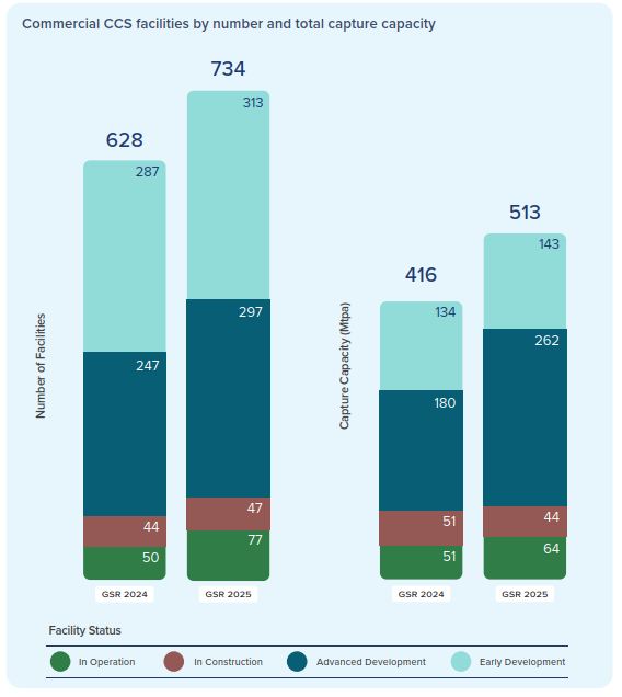
A consequence of this advancement is that plenty of engineers who’ve spent their careers keeping hydrocarbons flowing are about to be handed a very different fluid. We were invited to the SLB OLGA CCS Roundtable earlier this year as specialists with first-hand experience in modelling CCS, to present our findings and share what we’ve learned working with OLGA and its new NEO (Olga for New Energy Operations) solver, developed specifically for CCS systems. This piece is a distillation of what we brought to that table.
Same discipline, a very different fluid
Most of our readers are familiar with the traditional oil and gas playbook: multiphase flow where gas, liquid and water coexist and much of the job is managing that coexistence. Multiphase is a given; you design for it.
CCS flips the emphasis. For long-distance transport of CO2, the goal is to operate in the dense-phase and the primary reason is commercial: it packs liquid-like density into the pipe, so a single line can carry the tonnages of CO2 a project needs that it never could as a gas. Therefore, for a CCS export line, the whole point is to stay single phase. The moment it splits into two phases in a line that wasn’t designed for it, you inherit the entire hydrocarbon problem list (plus a few extra quirks unique to CO2) with none (or very little) of the tolerances to absorb it.
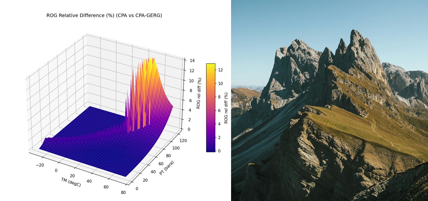
Here’s the part that makes CO₂ genuinely tricky, and it’s worth one good analogy. Picture a knife-edge mountain ridge. Out on the broad lower slopes where hydrocarbons live, you can walk ten metres in any direction and your altitude barely changes. The ground is forgiving. Now walk up to the razor ridge at the summit: one step left and you drop hundreds of metres into the liquid valley; one step right, the same plummet into the gas valley. A single pace is the difference between two different worlds.
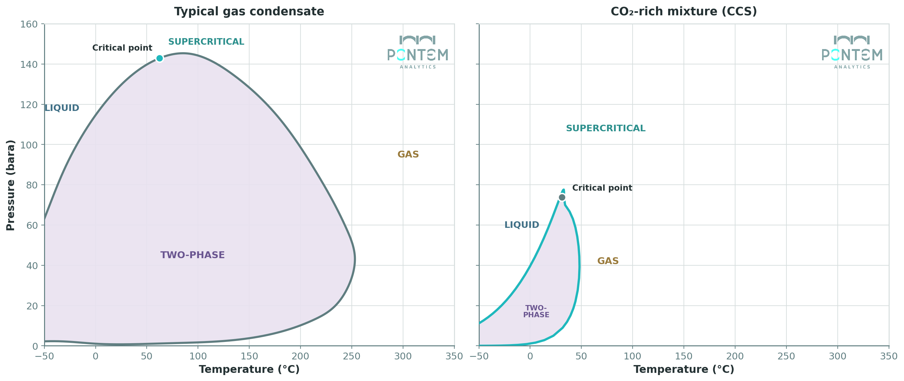
CO₂ operates right on that ridge, near its critical point (about 31 °C and 74 bar), where small changes in pressure or temperature can lead to dramatic changes in its properties. A model that’s “close enough” on the slopes can be catastrophically wrong up on the ridge, and the ridge is exactly where our fluid lives.
Get the fluid right first
So before we run a single simulation, we get the fluid model right - the EoS (equation of state) that tells the simulator how CO₂ behaves at every pressure and temperature it might see. Choose well and everything downstream stands on solid ground. Choose poorly and you’ve built a very expensive, very confident incorrect answer.
There’s a whole family of EoS to pick from, from fast, familiar workhorses (eg. RKSA and CPA) to high-accuracy models built for CO₂-rich mixtures with very specific sets of components (eg. GERG-2008, EoS-CG). On the gentle slopes (i.e. far from the critical point) they’re practically identical. However, up on the ridge they can potentially part ways. It’s the least exciting decision in the study and the one most likely to save a project. A quieter choice sits alongside it: feed the simulator a pre-computed property table, or make it solve the thermodynamics on the fly. We tested both - the fast option held up here, the gap only opening at very low flow rates.
Enter NEO
Which brings us to the guest of honour, and the reason our roundtable deck was called Into the Matrix.
NEO is the next-generation solver for OLGA, developed specifically to handle CO2, and in our experience, it’s been a genuine step change. Modelling a fluid this non-linear used to feel like trying to dodge bullets in slow motion. Numerical instability, regular crashes, and questionable results operating up on that ridge. NEO in conjunction with the new CO2 flow model (activated in OLGA by SOLVER=NEO, FLOWMODEL=OLGA, CO2=ON), handles the unique characteristics of CO2 with a stability and accuracy the older approach struggled to match. The difference between a model you trust and one you babysit.
The NEO solver is still in its early iterations and being such a new feature, it isn’t flawless, and pretending otherwise helps nobody. It is for these reasons that collaborating at industry events like the Roundtable that we presented at are important. At this event, we highlighted three specific examples from our own experience with NEO to follow up on: slugging in the dense phase, occasional non-convergence with the steady-state pre-processor, and flow instability at very low flow rates. None are a showstopper, and all are the kind of things you only find by pushing a numerical model hard against a real, challenging CCS problem.
NEO may be The One for CCS modelling, it’s just not done training yet (are any of us?).

Reading the Matrix: seeing the code behind the plot
Now assuming your fluid model and simulator have got the physics of living on that ridge correct, the final challenge is to interpret the results that are output from your simulations. If you’re coming from a traditional flow assurance background and familiar with multiphase hydrocarbon systems, the results for a CCS system can at times appear quite counter-intuitive and just plain wrong. This is where that red pill comes in.

For the analysis of hydrocarbon flow assurance, we mostly live on two kinds of charts: trend plots (values over time) and profile plots (values over distance along the pipe). They’re the right tools for oil and gas. For CCS, take the blue pill; keep using those traditional methods and the story looks calm, right up until a quirk you never saw coming bites you. This is because those plots don’t show where the fluid sits relative to the boundaries that matter - that ridge.
The red pill is to plot your operating conditions straight onto the phase envelope, so you can see at a glance how close you are to the bubble line, dew line, critical point, Widom line and hydrate curve. These results are then presented on a pressure-temperature (PT) plane that the system operates in, or for a more rigorous but perhaps less intuitive approach, on a pressure-enthalpy (PH) plane. However, we go one better, with what we call a PTH plot: overlay enthalpy contours across that pressure–temperature diagram, and now pressure, temperature and enthalpy all live in a single pane. The Nebuchadnezzar’s dashboard, if you like.
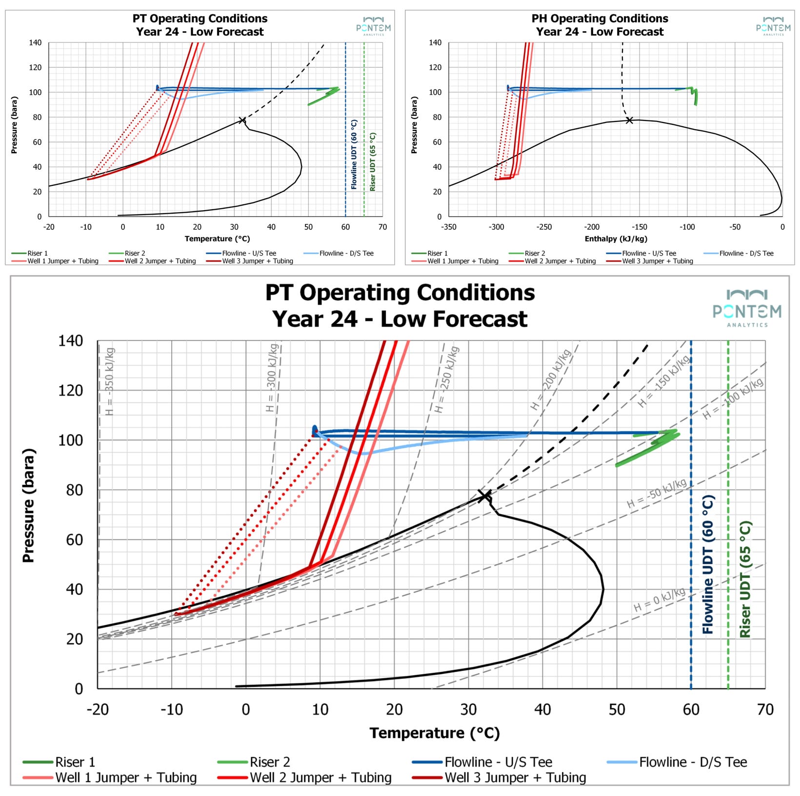
Remember the operators aboard that ship, reading the Matrix straight off the screen? Cascading green code to the uninitiated, “blonde, brunette, redhead” to them. A PTH plot is the same. A tangle of lines to those not familiar with this presentation method. However, once you’ve learned to read it, you see exactly where your fluid is and how much room it has before it does something you didn’t ask for. Free your mind, and the plot stops being a plot. There is no spoon.
Three glitches in the Matrix
Read the data this way and the “glitches” (results that make you doubt your model) resolve into explanations you can point at. Three specific examples we have encountered:
1. Hotter fluid when it’s colder outside. The mystery we opened with. Drop the ambient temperature and the CO₂ arrives at the bottom of the riser hotter. As the dense, heavy CO₂ descends the riser it compresses under its own weight, and with the rapid compression, heats up. That part is as expected. The twist is how much: a colder environment lowers the operating pressure in our system, and at lower pressure CO₂’s Joule–Thomson coefficient is higher. In other words, the temperature is more sensitive to a change in pressure. Same descent, bigger temperature rise. Cooler outside, warmer inside. Our PTH plots clearly show this phenomenon.
2. The −13 °C plunge. Late in field life our reservoir pressure reduces and tubing pressures are low enough that the fluid runs two-phase in our well tubing. CO₂’s Joule–Thomson coefficient is far larger in two-phase than in dense phase, so the temperature drop across the choke turns severe (rapidly plunging into sub-zero temperatures), once the operating point crosses the boundary. Again, the PTH plot shows the crossing; the moment we cross into the two-phase region and temperatures plummet. Real physics, not an artefact.
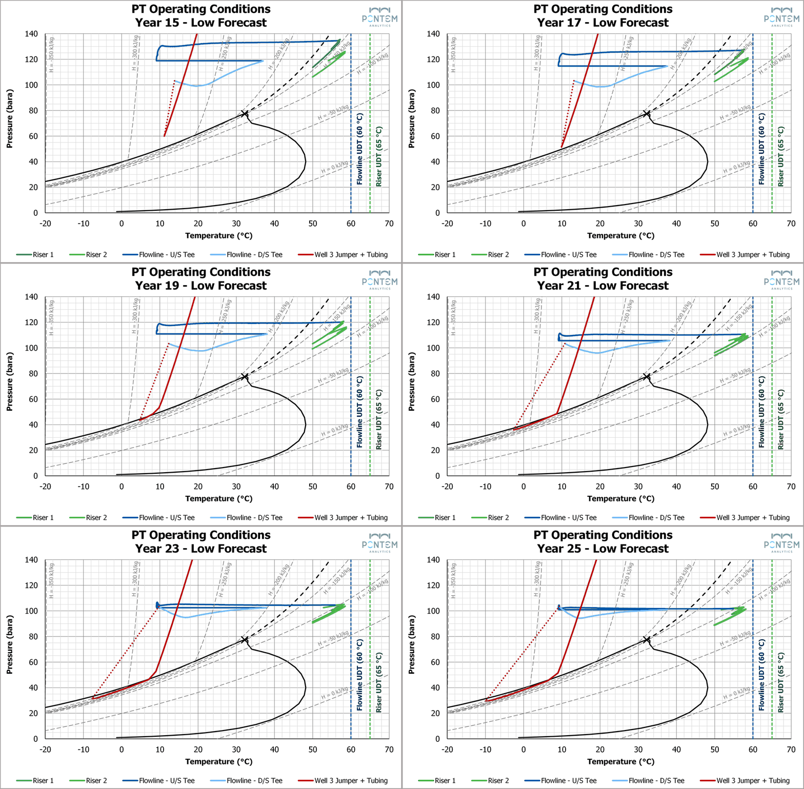
3. Flow-rate spikes. A flow-rate profile that jitters during steady-state operation for no good reason at all looks alarming. However, this one is numerics, not physics. As the fluid crosses the Widom line, OLGA flips how it labels the phase; all gas on one side, all liquid on the other, and that switch can introduce a discontinuity. Plot the operating point against the Widom line on a PTH plot and the spikes line up with the crossings.
The common thread with the three examples above? Knowing where you sit relative to the thermodynamic boundaries turns weird into explained. Sometimes that’s elegant physics; sometimes a numerical wrinkle to chase down. Either way, you can’t easily tell them apart until you can read the Matrix.
What we took away — and where we’re taking it next
Three things we’d write on the whiteboard. Get the fluid model right before you run anything; the cheapest couple of hours and the most expensive to skip. Visualise where you’re operating, not just what the numbers are. And treat NEO as the real step forward it is, while keeping a running list of its current limitations and known issues.
Thanks to all participants at the roundtable. Conversations like the ones held are how the industry’s tools get more features, faster and more stable performance, and most importantly, greater accuracy.
If this is your kind of thing, come and chat with us in person. We’ll be presenting on CCS flow assurance at the SPE Workshop “Beyond Boundaries — Advancing Cost-Effective and Sustainable Solutions in Flow Assurance,” 8–9 September 2026 in Kuala Lumpur, Malaysia. Fittingly there will be a session at the workshop dedicated to flow assurance for energy-transition fluids and CCS. If you’re there, we’ll be the ones talking about knife-edge ridges, cascading code and the absence of spoons.
Lots more to come. Stay tuned, and free your mind.
If you made it this far, thank you. Subscribe to Data and Discipline for more from the Pontem Analytics team on CCS, flow assurance, production chemistry, data analytics, and the occasional glitch in the Matrix.