
Emulsion Stability x Shear Rate
Replicating field conditions in the lab


My first trip offshore for a field trial included a baseline check on emulsion impacts. Understanding this was key to meeting our product and overboard specifications. This required mixing the fluids in our small, offshore lab in a way to replicate topsides boarding conditions, which basically amounted to ‘shaking vigorously’ several bottles. By creating a baseline similar to what the field was experiencing, this helped understand how our proposed changes would behave in the processing vessels.
Emulsions in oil & gas production are a bit like Dr. Jekyll and Mr. Hyde. In some instances, they can help reduce hydrate agglomeration tendencies and can keep pipelines “oil wet” to effectively inhibit corrosion. However, they increase viscosity in flow lines and impact separation, so ultimately, we don’t want them around. We want beautifully clear water and dry oil. In this post, we highlight a few fundamental emulsion properties and lessons learned to help answer the critical question when studying emulsions: how does a lab generate the same type of emulsion observed in the field? Let’s start with some fundamentals:
Emulsion Basics
An emulsion is a mixture of two normally immiscible fluids that exist as a dispersion of small droplets of one liquid into another. An illustration of two simple emulsions are shown below. The image on the right is a water-in-oil emulsion (w/o). The oil is the external or continuous phase, while the dispersed droplets are the water phase. This is the most common type of emulsion encountered in the oilfield. The image on the left is an oil-in-water (o/w). In the oilfield this is typically referred to as a reverse emulsion. The oil is now the dispersed phase and the water is the continuous phase.

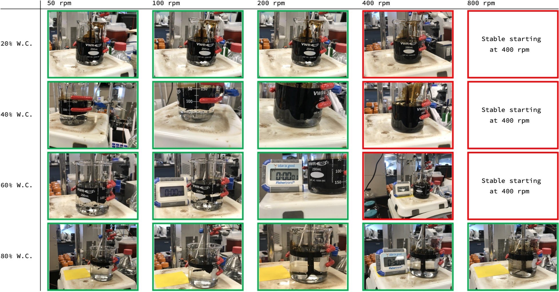
While not exhaustive, two variables that will impact emulsion formation and stability are shear rates and the volume of water in the system. An example of this can be seen in the bottle test comparisons below, where various emulsion breakers were tested in bottle tests at 40% water cut (top) and 70% water cut (bottom). In the 40% WC example, the emulsion is stable and two of the three chemicals are not effective at breaking the emulsion, while the third chemical is moderately effective. When water cuts are increased to 70%, the emulsion becomes unstable and even the blank separates into two clean phases.
In the next example, we looked at two low water cut scenarios and compared low and high mixing rates using Turbiscan technology to measure the light transmission through the water phase. This relies on a more quantitative technique, rather than the visual observations shown previously. In both scenarios, the high shear rates (HS trends) produced a more stable emulsion than the low shear rates (LS trends).

We’ll discuss shear rates in more detail below, however the important concept to recognize is the ability to reproduce field conditions when examining emulsion stability. With enough shear it is possible to create a highly stable emulsion with almost any oil and brine in the lab. The point is not to try and create the worst (most stable) emulsion possible. This is actually counterintuitive for many labs, as often is the case, the mindset is to look at the worst possible set of conditions and the testing needs to be robust, i.e., repeatable.
In the emulsion world, repeatable is most easily achieved with high shear rates to form a tight emulsion. A tight emulsion is one in which water droplets are very tiny, compared to a loose emulsion, which has larger water droplets. Typically, a loose emulsion is less stable as bigger droplets will more easily coalesce, which leads to fully separated oil and water phases. The ability to potentially create either type of emulsion for a given fluid could be related to the shear applied, which is something we will explore further.
There are many fluid properties that are impacted by emulsions, which will influence models used to predict production and operations scenarios. For example, increasing water cuts within a stable emulsion will increase the fluid’s viscosity. When an emulsion destabilizes resulting in two distinct, non-miscible phases the viscosity of the mixture will drastically decrease, generally approaching the viscosity of the external fluid medium (i.e. water, in an oil-in-water scenario).
In the example below, water cuts are increased in 10% increments while measuring fluid viscosity at various temperatures. While absolute viscosity values are different, the trends are similar: viscosity increases 5 - 6X up to 40% water cut. At higher water cuts, the emulsion destabilizes and the viscosity precipitously drops with increasing water cuts.

The emulsions above were created with an unknown shear, both because the values were not measured in the lab AND because they were not reported with the testing results, which makes it difficult to use the lab report later in design (i.e. lab work and design/engineering work, designed to produce field-ready recommendations, need to be tied together). Not knowing the shear relationship creates uncertainty whether the field will actually produce fluids with this viscosity profile. Hydraulic and process models are reliant on fluid properties, including emulsion viscosity, to generate accurate results. The old adage: Garbage In / Garbage Out. The consequences can be under/oversized pipelines, under/oversized equipment, lack of chemical injection , and failure to meet process guarantees. Let’s explore how we can do this and ensure a problem doesn’t occur:
You Bringin’ The Woelflin?! That’s All You Gotta Say…
Not exactly. There are a number of emulsion viscosity / water cut correlations reported in the literature. One particularly powerful one is the Woelflin dual constant equation. Briefly, the constants are used to describe an emulsion as tight or loose, which describes how big the dispersed phase droplets are. Tighter emulsions will have higher viscosities, in general.

The viscosity of stable emulsion can be examined in a rheometer in a series of shear rate ramp experiments. As water cuts increase, a shear-dependent viscosity vs water cut curve will develop, similar to the curves below for various oils. At a given shear rate, a best-fit curve analysis is conducted by changing the two constants in the equation. Ultimately, we see the viscosity of a fluid is quite dynamic and depends on the oil/water ratio, the stability of the emulsion (tight/loose), and the shear that generates the emulsion. The best-fit constants in the Woelflin equation can be used as input parameters to conduct hydraulic modeling using a tuned fluid.

It is worth noting that the graph above shows the viscosity vs. water cut behavior at a single temperature, with values increasing (log-scale) with water cut. Complicating this further, the testing may need to be carried out at multiple temperatures too, since the behavior also increases (log-scale) with lower temperatures. For the particular case study, the field happens to be north of the Arctic Circle, which means those -50°F data points become relevant, driving the need to capture the end-points in both (a) water cut and (b) temperature to generate a full-fluid rheology sweep.

Who Goes First: Oil or Water
Another important datapoint is the inversion point. This is the point in which emulsions will switch from oil-external to oil-internal. In the oilfield, most emulsions are oil-external. One simple way to think why this is relates to the fact that usually oil is produced first and eventually water breaks through as the field ages. Some will treat the inversion point as the point where the emulsion will become unstable and a free water phase forms. While the inversion point is important to consider, it is not the same as a destabilized emulsion.
Let’s take the example above in which water cuts above 40% resulted in unstable emulsions. In standard inversion point experiments following ASTM procedures conductivity is used to measure when the emulsion moves to water-external. Because oil does not readily conduct an electrical current, it is easy to determine when oil or water is the external phase. Additionally, the recommended procedure utilizes high shear mixing to generate a stable emulsion.
In the figure below, conductivity is measured in two separate methods: the top graph shows conductivity as water is added to the experiment. It is clear oil is external up to 70% water cut given the conductivity is less than 0.01 uS/cm. As water is added to 80% WC, a > 10x jump in conductivity indicating a change in external phase is occurring. Similarly, starting with 100% water and adding oil to the mixture, the lower graph is read right to left. The conductivity precipitously drops at 80% WC, indicating an external phase change from water-external to oil external.

This can be visualized in the video below. The beaker begins as a 90% WC emulsion and the conductivity is 27,760 uS/cm (note the units on the meter are mS/cm). As additional oil is added, the water cut is reduced to 81%. Watch the conductivity meter and pay attention to the units! The oil is fully added at the 0:12 mark. At the 0:32 mark, the conductivity drops to ~235 uS/cm! The reading fluctuates until 1:06 when another drop is noted and the conductivity stays below 75 uS/cm, indicating the mixture flipped from water external to oil external.
The reality is the field will rarely operate with sustained shear rates high enough to form a stable emulsion throughout the range of increasing water cuts (unless ESP’s or some other high shear equipment is involved). What typically happens is field shear rates will form stable emulsions up to a much lower water cut than the inversion point. When emulsions destabilize, a free water phase results.
Solids Impact
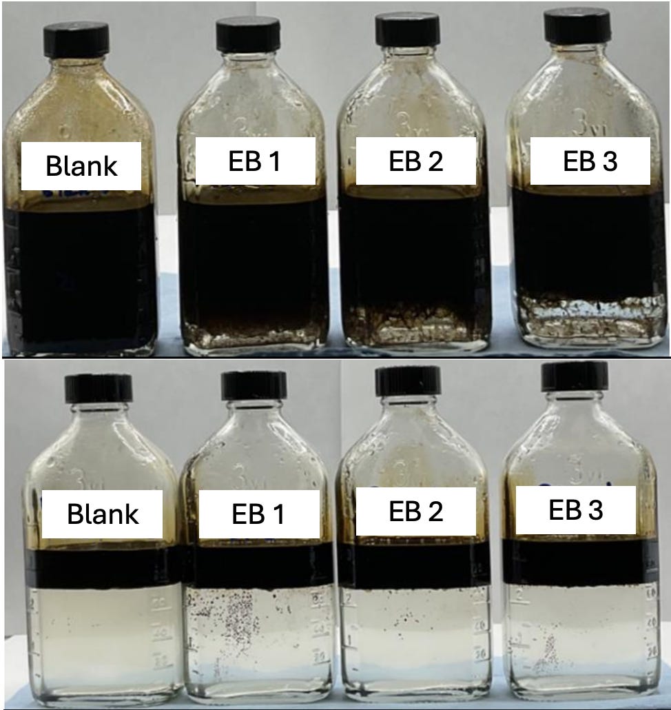
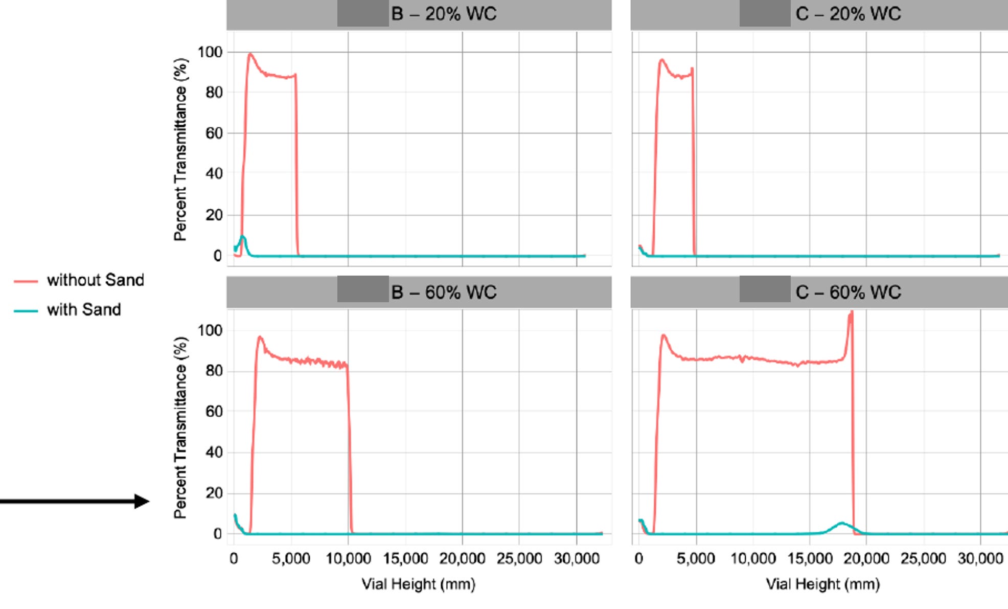
We further evaluated the effect of proppant on stabilizing emulsions, particularly during early production periods as we brought new wells into the system. Using Turbiscan transmittance as a guide, we were able to see that inclusion of sand (to represent the expected proppant particle sizes) was very effective at stabilizing emulsions. The lack of transmittance change in the graphs below indicate no phase separation in the cases with sand, but clear separation without.
Additionally, visual observations clearly show oil coating of the proppant (sand), again highlighting the importance of considering a “real” system (contaminants and all) when carrying out any lab testing.

Shaken, Not Stirred
We alluded to the following earlier, however it is worth highlighting again for this discussion. Different emulsions will form with different shear rates:
High shear - repeatability in measurement, small droplets, generally stronger emulsions, generally higher inversion point
Low shear - more akin to expected field conditions, harder to maintain consistency (repeatability), often subject to ‘bottle shaker’ technique
It is also important to recap how we’ve progressed:
Emulsions are important to understand because they can impact fluid properties like viscosity
Different oils and waters, their ratios, and shear rates will form different emulsions with different viscosities
Best practices will take into account the expected or known shear rate from the field and use that as the basis to form emulsions on the bench top
Hand shaking bottles will generate lower but unknown shear rates, impeller-type homogenizers will generate high shear and over emulsified fluids, and overhead mixer can provide variable shears however mixing speeds are set via rpm (revolutions per minute). How then do we correlate rpm to shear rates to make a representative emulsion in bulk?
We decided to investigate this last point: correlating what we do in the lab with what we expect in the field. Because fluid velocities (and hence shear rates) are not uniform in an overhead mixer set-up, we ran a Computational Fluid Dynamics (CFD) analyses to mirror our bench-top experimental set-up. Check out the video. As the analysis goes up the z-axis, the shear rates change dynamically throughout the beaker, showing a truly dynamic set of conditions within a single test.
Under various water cuts and mixing speeds (RPM), we were able to generate shear rate profiles for the experimental set up. We isolated several fixed z-axis points and averaged shear rates in those 2-D sections to calculate and overall shear rate for a given set of conditions. We can now examine specific shear rates under laboratory conditions that approximate actual field condition values. By doing this, we can predict whether the field will produce a stable emulsion at expected operating conditions, and if so, can use the resulting fluid viscosities in hydraulic modeling and plan operations accordingly to handle fluid separation processes.
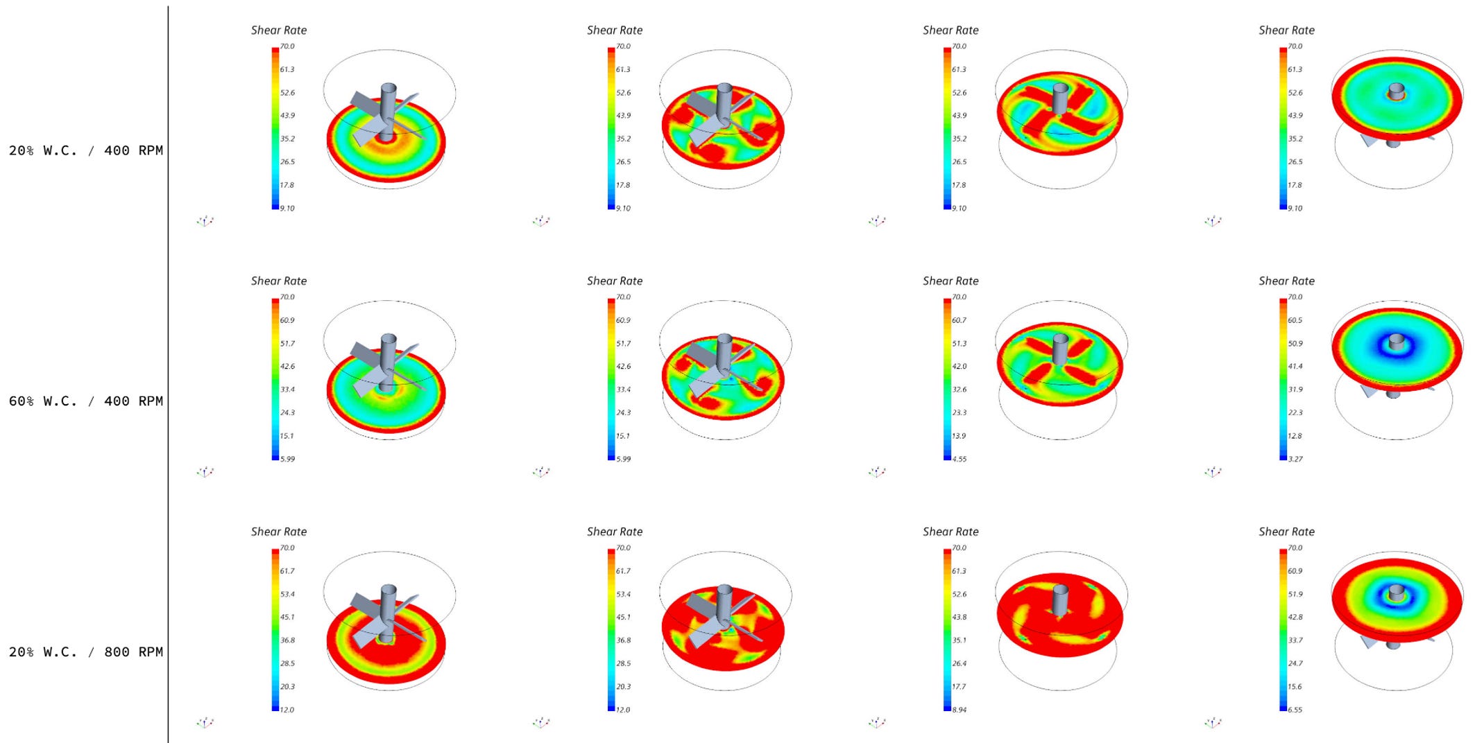
The full visual data set is shown below. It is worth noting this study was examining conditions for two separate well / flow line configuration. The results indicated one flow line would likely form emulsions under representative field shear rates, while the second production scenario would not, which was relevant because - on the surface - both configurations looked “similar”.
Closing Thoughts
Emulsions are important to consider upstream of separation vessels of the production train. While obtaining fully separated oil and water is the ultimate goal, the emulsions that form in the pipeline and downhole tubing will impact hydraulics, as well as other issues not covered here, such as corrosion risks. Hopefully, this discussion provides a good jumping off point to dig further into! There are other considerations that will influence emulsion stability, such as oil-based muds or proppants that flow back during initial well start-ups. While these factors can be transient, they are important to consider. Lastly, we’ll close with emulsions will resolve with enough time and heat…if you don’t have enough of either, reach out to Pontem and we’ll be happy to look into your system for solutions to break your emulsions!